RoboSoccer Unscented Kalman Filter Localization with Field Line Observations (2022-2023)

Estimating the visual odometry pose

Since we are dealing with particles rather than individual lines, the processing tends to be computationally expensive. However, the trade-off is possible since we use UKF rather than the much more computationally expensive particle filter.

The first part of the algorithm is to detect the closest line to a point. By first computing the distances for every particle to every single line, we match every single line with the closest line. There are certain exceptions to this.

• If the point is too far from any single line, it is not considered matching with any line.

• If the point is equidistant with two lines, such as in the corner between the field, then it can be included as part of both lines or can be excluded from the detection.

Next, the average distance of every single point to its closest line is calculated, because the particles have a spread equivalent to the width of the line, then the average distance from every particle to the center of the field line will successfully match the points onto the field line in the best way possible. Using the average x and y distance the estimated location according to odometry $T_{odom}$ is calculated.

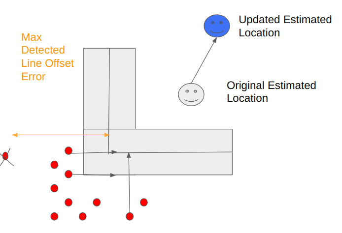
Each point from the field line is transformed to a point cloud situated on the ground plane

For rotation the method is more challenging, See Figure below. First, a central location for all particles is calculated. represented as the orange point. Next, every single point is projected to its closest line, and the angle between the moved point and the final point is calculated. By summing up the average angle, we get the average rotation of the point cloud to its corresponding line.

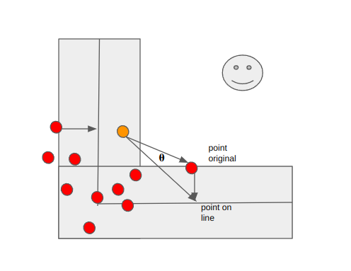
Each point from the field line is transformed to a point cloud situated on the ground plane

Now that we have the average ${\Delta{x}, \Delta{y}, \Delta{\theta}}$ we use this transformation on top of the original estimated pose to get an Odom estimated pose.

Combining the visual odometry pose with the Unscented Kalman Filter

The Unscented Kalman filter (UKF) combines odometry measurements calculated from robot movement odometry and the odom estimated pose to produce an optimal estimate. The Unscented Kalman filter was chosen because of its simplicity and robustness to highly nonlinear movements, as opposed to an extended Kalman filter (EKF), which requires that the robot model’s nonlinear equations be accurate.

The predict step of the unscented Kalman filter uses the provided odometry value to extrapolate to the next state. The basic nonlinear robot movement equation uses the previous state and the newly provided odometry value, since the $x$, $y$, and $\theta$ differences are provided in the odometry estimates, it is a simple extrapolation.

The update step uses the previously calculated odometry value and then uses the point cloud to line-matching algorithm as mentioned in the section above to calculate an accurate location of the robot.

Since the Kalman filter uses an unscented transform, the previous uncertainties can be used to calculate the sigma points. These points are applied through the predict and update steps to calculate the new covariance values post-transform. If sufficiently reasonable estimates are provided for odometry error and visual odometry error, where visual odometry error is assumed to be much larger. Then the robot is able to navigate to the destination with good accuracy. The tuning of the covariance parameters for the predict and update steps is largely based on keeping the ground truth within the 1 sigma bound, as it is infeasible to analytically calculate the covariance from the computer vision model.

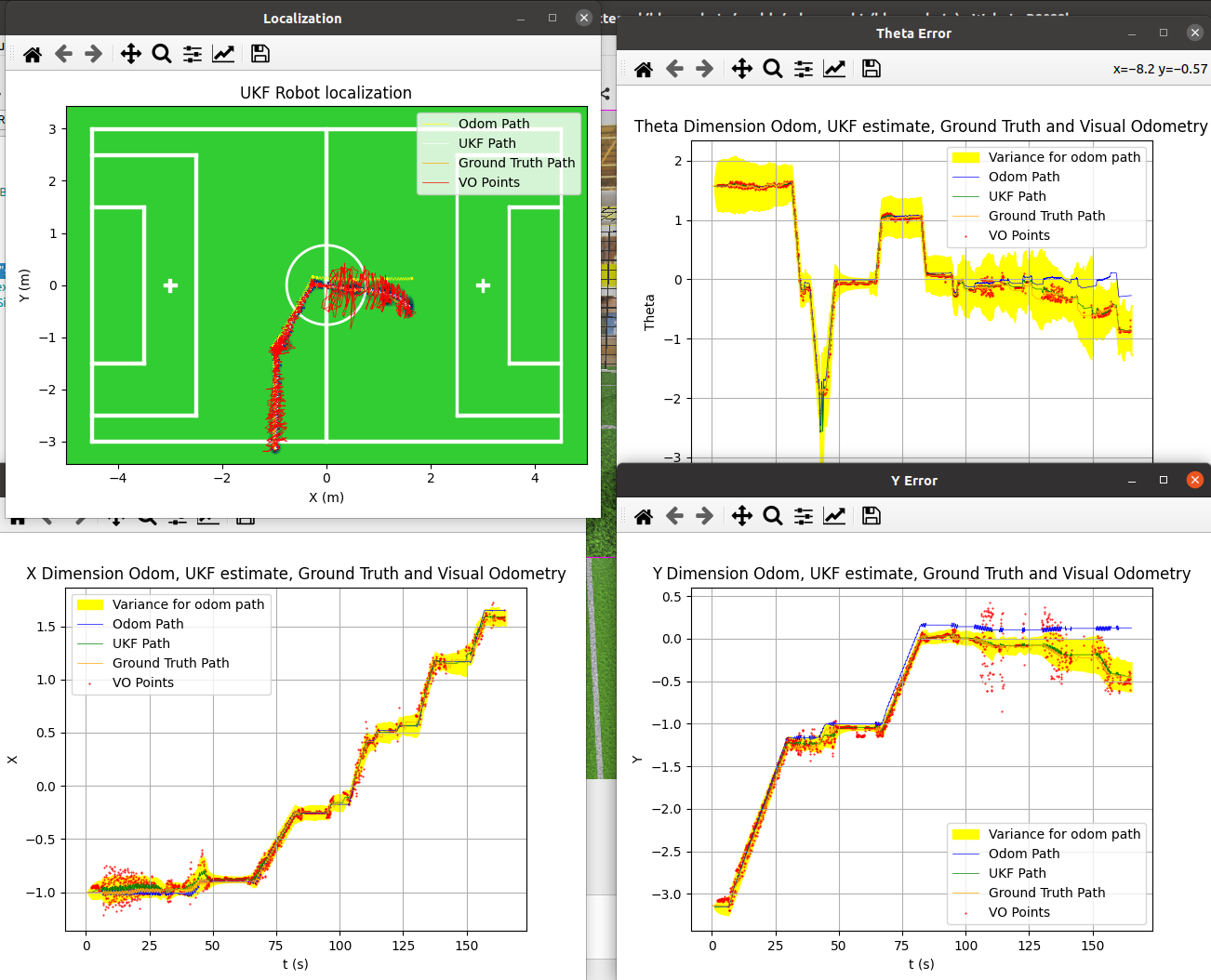
Results for Unscented Kalman Filter (UKF)

Video